Use of a new crop variety or production technique may dramatically increase food production in a given area. Alternatively, an innovation successful in North America may utterly fail in the tropics. The goal of “adaptive research” is to evaluate a particular innovation for its usefulness under local conditions. This technical note is written for those who want to improve the quality of their experiments but who have little or no background in statistics. It supplements the 81st issue of ECHO Development Notes with step-by-step instructions on how to manually calculate statistics for the most commonly used experimental designs. A little persistence, very basic math skills, and perhaps a calculator are all you need to do the calculations. If you have a computer equipped with statistical software, doing a set of calculations by hand or with a calculator will help you to understand how to use the software and interpret the output. Examples are given for experiments in which only one factor (e.g. crop variety) is tested. A limited amount of statistical terminology is woven into the text for the benefit of those interested in further study.
Example 1: Comparison of two averages using a T-test
A T-test could be used to determine, for example, if the average tomato fruit weight of variety A is similar to that of variety B. T-tests can also be used for analyzing survey results. In doing a T-test, standard deviation from an average is also calculated.
Imagine a farmer’s field in which we had randomly selected and harvested three rows each of tomato variety A and B. Table 1 contains the yield data collected from each of six rows (10 plants per row). A T-test would tell us if there is a statistical difference between the average yield of variety A vs. that of variety B. Steps 1 to 3 below illustrate how to calculate the numbers in the bottom 3 rows of Table 1 that are then used in steps 4 to 8 for a T-test. The “null hypothesis” (see EDN 81) tested is that the average yields are similar.
|
Table 1. Total fruit production with two tomato varieties. |
||
|
Total fruit weight (Kg/10 plants) |
||
|
Variety A |
Variety B |
|
|
30 |
40 |
|
|
25 |
45 |
|
|
28 |
38 |
|
|
Number of observed values |
3 |
3 |
|
Average of observed values |
27.67 |
41.00 |
|
Standard deviation |
2.52 |
3.61 |
- Count the number of observed values (weights) for each variety. In this case, three values were measured for each variety.
- Calculate the average of the three values for each variety.
Average for variety A = (30 + 25 + 28)/3 = 27.67
Average for variety B = (40 + 45 + 38)/3 = 41.00
- Calculate the “standard deviation” of the average weight for each variety. A small value for standard deviation is desirable because it tells you that the individual values (e.g. 30, 25, and 28 for variety A shown in Table 1) are all quite close to the average (27.67 for variety
A). Steps to calculate the standard deviation for variety A are as follows:
A. Subtract the average (27.67) from each of the three values (30, 25, and 28).
30 – 27.67 = 2.33
25 – 27.67 = -2.67
28 – 27.67 = 0.33
B. Square (multiply a value by itself) each difference calculated in step 3A.
2.33 X 2.33 = 5.43
-2.67 X –2.67 = 7.13
0.33 X 0.33 = 0.11
C. Add up the values resulting from step 3B.
5.43 + 7.13 + 0.11 = 12.67
D. Subtract 1 from the number of observed values (3).
3 – 1 = 2.
E. Divide the sum from step 3C (12.67) by the number from step 3D (2).
12.67/2 = 6.34 (this number is called the “sample variance”)
F. The standard deviation for variety A is equal to the square root of 6.34.
√6.34 = 2.52
G. Repeat steps 3A to 3F to calculate the standard deviation (3.61) for variety B.
- Obtain what is called the “common variance”.
A. Subtract 1 from the number of values for variety A. Recall from step 1 that 3 values were obtained for each of the varieties.
3 – 1 = 2
B. Multiply the result of step 4A (2) by the square of the standard deviation (2.52; see step 3) for variety A.
2 X 2.522 = 12.70
C. Repeat steps 4A and 4B for variety B. Recall that the standard deviation for variety B was 3.61 (see step 3).
Repeat of step 4A for variety B: 3 – 1 = 2
Repeat of step 4B for variety B: 2 X 3.612 = 26.06
D. Add up the values calculated in steps 4B and 4C.
12.70 + 26.06 = 38.76
E. Subtract 2 from the total number of values (3 for variety A + 3 for variety B = 6).
6 – 2 = 4
F. Divide the result of step 4D by that of step 4E.
38.76/4 = 9.69 (this is the common variance)
- Calculate the “standard deviation of the difference between means” (only need to know that this is not the same thing as described for step 3) using the common variance (9.69; step 4).
A. For each variety, divide 1 by the number of values obtained for that variety. Recall that 3 values were obtained for each variety. Add the resulting numbers together.
Variety A: 1/3 = 0.33
Variety B: 1/3 = 0.33
0.33 + 0.33 = 0.66
B. Multiply the result of step 5A (0.66) by the common variance (9.69).
0.66 X 9.69 = 6.40
C. Calculate the square root of the result of step 5B (6.40).
√6.40 = 2.53 (the standard deviation of the difference between means)
- Obtain a value for “calculated T”.
A. Subtract the average weight of variety A from the average weight of variety B.
27.67 – 41.00 = -13.33
B. Divide the result of step 6A (-13.33) by that of 5C (2.53).
-13.33/2.53 = -5.27
Use the absolute value of –5.27, so your calculated T statistic is 5.27.
- Obtain a “critical T” value from Table 5 shown near the end of this article. The far-left column of the table contains numbers from 1 to infinity (∞) known as “degrees of freedom”. Degrees of freedom for a T-test are calculated by subtracting 2 from the total number of values (see step 4E). In this case, therefore, we have 4 (3 + 3 – 2) degrees of freedom.
At the top of each column of Table 5, you will see significance levels ranging from 40% (0.4) down to 0.05% (0.0005). A significance level of 5% is usually considered acceptable. In choosing a significance level of 5%, we are willing to accept a 5% chance of being incorrect if we reject the null hypothesis and, thereby conclude that the average weight for variety A is different from that for variety B. Conversely, we will be 95% (100% -5%) certain of being correct in our conclusion. A significance level of 5% also means that the P (probability; see EDN 81) value is less than or equal to 0.05. Exact P values are difficult to calculate manually.
Critical T, in this case, is 2.132 intersected by the row of numbers across from 4 degrees of freedom and the column of numbers under the significance level of 0.05.
- Compare “calculated T” (5.27) vs. “critical T” (2.132) to determine if the average tomato weight for variety A differs from that for variety B. If “calculated T” is greater than “critical T”, then there is a significant difference between the two averages being tested. If “calculated T” is equal to or less than “critical T”, then the two averages are statistically similar. In Example 1, the value of 5.27 exceeds 2.132, so we reject the null hypothesis and conclude that the total tomato weight for variety A (27.67) is less than that for variety B (41.00).
NOTE: A T-test could also be used for analyzing results of surveys in which a single factor (e.g. yield) is tested. For instance, suppose we had obtained maize yield data from farmers who A.) used fertilizer and B.) had not used fertilizer. The data would be analyzed similarly as in Example 1 by substituting farmer groups for tomato varieties. I suggest investigating the use of chi-square tests for more elaborate surveys where more than one factor is tested.
Example 2. Analysis of qualitative data with a Completely Randomized Design
In Example 1, we were simply interested in testing marketable yield of two tomato varieties. What would we need to do if we were interested in testing more than two varieties? The statistically correct way to handle this situation is a procedure called analysis of variance (ANOVA), and experiment design becomes important when doing ANOVA.
A CRD is used when the experiment is conducted in a small area such as a shade house bench or a small, uniform plot of ground. Consider the pumpkin variety trial illustrated in EDN 81, a single-factor (crop variety) experiment in which three pumpkin varieties were tested: 1.) La Primera, 2.) Butternut, and 3.) Acorn. Each of the three varieties were evaluated (replicated) three times, so 9 (3 varieties X 3 reps) planting beds were made with each bed long enough for 6 pumpkin plants. Each of the 9 beds had an equal (random) chance of receiving either of the 3 varieties (see EDN 81 for information on how to randomize). Let us assume that the varieties were planted in the field in a CRD as shown below:
|
Bed 1 Acorn |
Bed 4 Acorn |
Bed 7 Butternut |
|
Bed 2 Butternut |
Bed 5 Butternut |
Bed 8 La Primera |
|
Bed 3 La Primera |
Bed 6 La Primera |
Bed 9 Acorn |
We will use the same data (Table 2A below) as in EDN 81 in testing the null hypothesis that there are no differences between average yields (20.1, 6.72, and 11.4).
|
Table 2A. Yield (kg fruit per 6 plants) data for tropical pumpkin variety trial. |
|||||
|
Variety |
Replicate 1 |
Replicate 2 |
Replicate 3 |
Totals |
Averages |
|
La Primera |
21.10 |
17.90 |
21.20 |
60.20 |
20.10 |
|
Butternut |
4.42 |
2.95 |
12.80 |
20.17 |
6.72 |
|
Acorn |
15.20 |
5.78 |
13.10 |
34.08 |
11.40 |
|
Grand total = |
114.45 |
||||
In doing ANOVA, an “F” instead of a “T” value will be calculated by doing the following steps:
- For each variety, sum the values obtained in the three replicates (beds).
La Primera: 21.10 + 17.90 + 21.20 = 60.20
Butternut: 4.42 + 2.95 + 12.80 = 20.17
Acorn: 15.20 + 5.78 + 13.10 = 34.08
See these numbers entered in the “Totals” column of Table 2A.
- Sum the numbers obtained in step 1 (60.20, 20.17, and 34.08).
60.20 + 20.17 + 34.08 = 114.45 (shown as “Grand total” in Table 2A)
- Calculate “total sum of squares” abbreviated as SST.
A. Square each of the 9 values and add the resulting numbers together.
21.12 + 4.422 + 15.22 + 17.92 + 2.952 +5.782 + 21.22 + 12.82 + 13.12 = 1843.20
B. Square the grand total (114.45 in Table 2A) and divide the resulting number by the total number of values (9).
114.452/9 = 1455.42
C. Subtract the result of step 3B (1455.42) from that of step 2A (1843.20).
1843.20 – 1455.42 = 387.78
Thus, SST = 387.78
- Calculate treatment sum of squares abbreviated as SSTreatments
A. Square the 3 values (60.2, 20.17, and 34.08; not the “Grand Total”) in the “Totals” column of Table 2A; see step 1 for how these were obtained. Add up the results.
60.22 + 20.172 + 34.082 = 5192.32
B. Divide the previously obtained value (5192.3153) by the number of replicates (3).
5192.3153/3 = 1730.77
C. Subtract the value obtained in step 3B (1455.42) from that in step 4B (1730.77).
Thus, SSTreatments is equal to 1730.77 – 1455.42 = 275.35
- Calculate the “error sum of squares” abbreviated as SSE by subtracting the value for
SSTreatments (275.35) from that for SST (387.78).
SSE = 387.78 – 275.35 = 112.43
- Calculate “degrees of freedom” for SSTreatments, SSE, and SST. Two easily-obtained numbers identified as “a” [number of levels of a factor (“variety” in Example 2)] and “N” (total number of values) are required. Three varieties were tested, so “a” is equal to 3 (same as the number of averages). “N” is equal to 9 because there were 9 measured values in Example 2.
A. Degrees of freedom for SSTreatments = a – 1
= 3 –1 = 2
B. Degrees of freedom for SSE = N - a
= 9 – 3 = 6
C. Degrees of freedom for SST = N - 1
= 9 – 1 = 8
- Calculate “mean squares” abbreviated as MSTreatments and MSE.
A. MSTreatments = SSTreatments /Degrees of freedom for SSTreatments
= 275.35/2 =137.68
B. MSE = SSE /Degrees of freedom for SSE
= 112.43/6 = 18.74
- Obtain a calculated F value by dividing MSTreatments (137.68) by MSE (18.74).
Fcalculated is equal to 137.68/18.74 = 7.35
HINT: Make an ANOVA table (below) to help you understand steps 1 to 8.
|
Table 2B. Analysis of variance table describing information needed for a CRD. |
||||
|
Source of variationZ |
Sum of squares |
DFY |
Mean Square |
FCalculated |
|
Between treatments |
SSTreatments |
a - 1 |
MSTreatments |
MSTreatments/ MSE |
|
Error within treatments |
SSE |
N - a |
MSE |
|
|
Total |
SST |
N - 1 |
|
|
|
ZA CRD accounts for variation between and within treatments (varieties). |
||||
|
YDF = degrees of freedom; see step 5 of Example 2 for definitions of “a” and “N”. |
||||
|
Table 2C. Analysis of variance table with information for Example 2. |
||||
|
Source of variation |
Sum of Squares |
DFZ |
Mean Square |
FCalculated |
|
Between treatments |
275.35 |
2 |
137.68 |
7.35 |
|
Error within treatments |
112.43 |
6 |
18.74 |
|
|
Total |
387.78 |
8 |
||
|
ZDF = degrees of freedom |
||||
- Obtain a critical F value. This is done using an F distribution table.
A. Select an “F distribution table” corresponding to your desired significance level. Table 6 at the end of this document contains F values for a significance level of 5%.
B. Calculate degrees of freedom corresponding to the “numerator” (MSTreatments) and “denominator” (MSE) of “F”. The terms “numerator” and “denominator” are used because “F” is a ratio, in this case of MSTreatments/MSE.
1.) Degrees of freedom for “numerator” = a –1 with a equal to 3 (see step 6A)
3 – 1 = 2
2.) Degrees of freedom for “denominator” = N – a with N equal to 9 (see step 6B and a equal to 3 (see step 6A)
9 – 3 = 6.
C. Fcritical in Table 6 is 5.14, the value intersected by the column of numbers under 2 degrees of freedom for the numerator and the row of numbers across from 6 degrees of freedom for the denominator.
- Decide if the average yields are similar to or different from one another. If FCalculated is greater than FCritical, then the averages are not similar. In example 2, FCalculated (7.35) exceeded FCritical (5.14). Therefore, with 95% certainty, we can say that not all the average marketable yields were similar.
- Make comparisons between averages. Steps 1 to 10 illustrated how to determine that differences between averages exist. This step will illustrate a simple test used to determine how the averages differ. We want to know, for instance, if the yield from La Primera differs significantly from that with Butternut. There are many tests that can be used, but one called “least significant difference” is commonly reported in literature and is calculated as follows:
A. Decide which significance level you will accept and divide that by 2. Let us use a significance level of 5% (expressed as a number, 5% is 0.05).
0.05/2 = 0.025
B. Note the degrees of freedom associated with MSE- in this case, 6 (see Table 2C). This number, as well as the result of 11A, is required to obtain a critical T value as described in the following step.
C. Obtain the critical T value (2.447) in Table 5 intersected by the column of numbers under a significance level of 0.025 (step 11A) and the row of numbers across from 6 degrees of freedom.
D. Multiply MSE (18.74; see step 7B) by 2.
18.74 X 2 = 37.48
E. Divide the result of the previous step (37.48) by the number of values used to calculate each average (3).
37.48/3 = 12.49
F. Calculate the square root of the value obtained in step 11E (12.49).
√12.49 = 3.53
G. Multiply the result of step 11C (2.447) by that of step 11F (3.53).
2.447 X 3.53 = 8.64
In Example 2, therefore, the LSD value used to determine if any two averages are statistically different is 8.64. If the difference (absolute value) between any two averages is greater than 8.64, the two averages are not the same. For example, we would want to make the following comparisons using the average yields in Table 2:
La Primera vs. Butternut: 20.10 – 6.72 = 13.28; 13.28 > 8.64 so these averages differ.
La Primera vs. Acorn: 20.10 – 11.40 = 8.7; 8.7 > 8.64 so these averages differ.
Butternut vs. Acorn: 11.40 – 6.72 = 4.68; 4.68 < 8.64 so these averages do not differ.
Example 3. Comparison of averages when treatments are “quantitative”
In Example 2, the treatments tested are “qualitative” because one cannot measure or quantify “tomato variety”. One can, however, measure “quantitative” factors such as rate (e.g. fertilizer, plant density/spacing, temperature, or time after crop establishment). Example 3 illustrates an accepted method of characterizing yield response to a factor such as rate.
Consider an experiment in which we obtained the exact same data as shown in Example 2. Instead of testing pumpkin varieties, suppose we had tested several rates of a herbicide to find out if it can be sprayed over pumpkin plants without injuring the crop. It is important to choose rates that are “equally spaced” to avoid the need for computer software to analyze the data. For instance, the numbers 0, 25, and 75 are not equally spaced because there is a difference of 25 between 0 and 25 and a difference of 50 between 25 and 75. Suppose we had chosen rates of 0, 5, and 10 liters herbicide/plot. Table 2A would then become Table 3A below:
|
Table 3A. Pumpkin yield (kg fruit per 6 plants) with 3 herbicide rates. |
|||||
|
Herbicide (L/plot) |
Replicate 1 |
Replicate 2 |
Replicate 3 |
Totals |
Averages |
|
0 |
21.10 |
17.90 |
21.20 |
60.20 |
20.10 |
|
5 |
4.42 |
2.95 |
12.80 |
20.17 |
6.72 |
|
10 |
15.20 |
5.78 |
13.10 |
34.08 |
11.40 |
|
Grand total = |
114.45 |
||||
To analyze the data in Table 3A, proceed as follows:
- Do ANOVA because there are more than two averages to compare [Note: if the only rates tested were 0 and 5, then we would only need to conduct an F-test (Example 2) to find out if yield with the 0-liter rate was less than or similar to that with the 5-liter rate]. In this case, we have already done the ANOVA in steps 1 to 10 of Example 2. We know there are differences between the averages. We still need to know how pumpkin yield responded to herbicide rate.
The graph (Figure 1) below represents the data in Table 3A. Notice, for example, that there are 3 dots (data points) directly above “5” (herbicide rate). These three points correspond to values 4.42, 2.95, and 12.8 in Table 3A. It appears that there are only 2 points above the “0” rate because two values (21.10 and 21.20) were almost the same. The object is to define a line that can be drawn through the points in Figure 1.
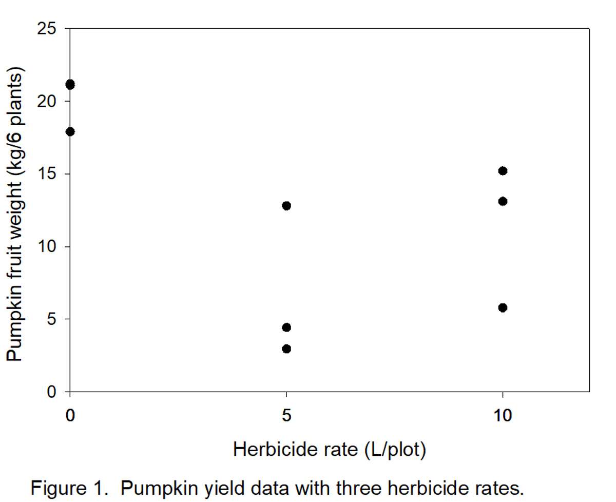
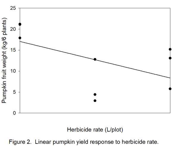
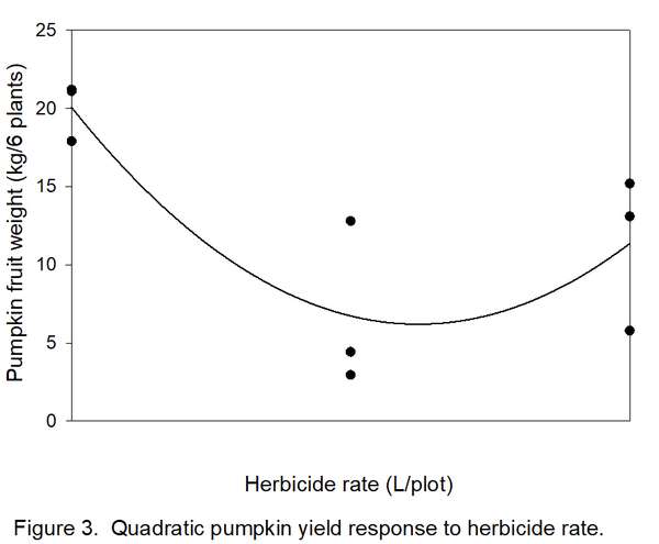
- Determine how many types/shapes of lines are possible by subtracting 1 from the number of rates (3 – 1 = 2). Thus, two line shapes will be tested. The most commonly used line shapes are linear (always the first possibility) and quadratic (always the second possibility). There are more line shapes, but these do not always make biological sense. We want to know if yields decreased linearly (Figure 2) or quadratically (Figure 3) with increased herbicide.
- Obtain “orthogonal coefficients” for each line shape from Table 7 on page 20. The rates (0, 5, and 10 liters/plot) we used are orthogonal because they were equally spaced (difference of 5 liters between each rate). If they had not been equally spaced, we could not use the coefficients in Table 7. Find coefficients for 3 levels of a factor (rate in this case) because we tested 3 rates.
Coefficients for testing significance of a linear line: -1, 0, 1
Coefficients for testing significance of a quadratic line: 1, –2, 1
NOTE: The three numbers for each line shape add up to zero. Making sure your coefficients add up to zero is a quick way to be sure you have the correct numbers.
- Calculate the “contrast estimate” for a linear and quadratic line using the coefficients obtained in step 3 and the average yield (20.1, 6.72, and 11.4) obtained with each herbicide rate. Abbreviations below are “AY” for average yield, “w/” for with, and “L” for liters.
A. For a linear line = (-1 X AY w/ 0 L) + (0 X AY w/ 5 L) + (1 X AY w/ 10 L)
NOTE: The first number in each set of parentheses is one of the three coefficients listed in step 3 for a linear line. Notice that they are used in the order that they appear in step 3: the first coefficient (-1) is multiplied by the first herbicide rate (0 L); the second coefficient (0) is multiplied by the second rate (5 L); and the third coefficient is multiplied by the third rate (10 L). Thus, the contrast estimate for a linear line is calculated as follows:
= (-1 X 20.1) + (0 X 6.72) + (1 X 11.4)
= -20.1 + 0 + 11.4
= -8.7
B. For a quadratic line = (1 X AY w/ 0 L) + (-2 X AY w/ 5 L) + (1 X AY w/ 10 L)
NOTE: The first number in each set of parentheses is now the appropriate coefficient for testing the significance of a quadratic line. Plugging in values for average yield (AY):
= (1 X 20.1) + (-2 X 6.72) + (1 X 11.4)
= 20.1 + (-13.44) + 11.4
= 20.1 – 13.44 + 11.4
= 18.06
- Calculate the sum of squares for each line shape using the formula:
Sum of squares = (number of replications per treatment X (contrast estimate2)/sum of squares of the coefficients
There were 3 replications per treatment, and contrast estimates were calculated in the previous step. “Sum of squares of the coefficients” is found by squaring each coefficientand summing the resulting values. The sum of squares of the coefficients is equal to 2 (-12 + 02 + 12) for testing the significance of the linear line and 6 (12 + -22 + 12) for testing the significance of the quadratic line. Therefore, the sum of squares for the linear and quadratic line are calculated as follows:
A. Sum of squares for linear line = (3 X –8.72)/2
= (3 X 75.69)/2
= 113.54 (we will call this value SS1)
B. Sum of squares for quadratic line = (3 X 18.062)/6
= (3 X 326.16)/6
= 163.08 (we will call this value SS2)
- For each line shape, calculate a value for “F” by dividing the sum of squares (see step 5A for linear line; step 5B for quadratic line) step 5 by MSE (18.74 used for both line shapes) as already calculated in Example 2 and shown in Tables 2B and 2C):
A. FCalculated for the linear line: 113.54/18.74 = 6.06
B. FCalculated for the quadratic line: 163.08/18.74 = 8.70
Tables 3B and 3C illustrate how to make an ANOVA table with results of steps 1 to 6.:
|
Table 3B. Analysis of variance table describing information needed for Example 3. |
||||
|
Source of variationZ |
Sum of squares |
DFY |
Mean Square |
FCalculated |
|
Between treatments |
SSTreatments |
a - 1 |
MSTreatments |
MSTreatments/ MSE |
|
Linear line |
SS1 |
1 |
Same as SS1 |
SS1/ MSE |
|
Quadratic line |
SS2 |
1 |
Same as SS2 |
SS2/ MSE |
|
Error within treatments |
SSE |
N - a |
MSE |
|
|
Total |
SST |
N - 1 |
|
|
|
ZA CRD accounts for variation between and within treatments (varieties). |
||||
|
YDF = degrees of freedom; see step 5 of Example 2 for definitions of “a” and “N”. |
||||
|
Table 3C. Analysis of variance table with information for Example 2. |
||||
|
Source of variation |
Sum of Squares |
DFZ |
Mean Square |
FCalculated |
|
Between treatments |
275.35 |
2 |
137.68 |
7.35 |
|
Linear line |
113.54 |
1 |
113.54 |
6.06 |
|
Quadratic line |
163.08 |
1 |
163.08 |
8.70 |
|
Error within treatments |
112.43 |
6 |
18.74 |
|
|
Total |
387.78 |
8 |
||
|
ZDF = degrees of freedom |
||||
- Determine a critical F value for a significance level of 5%. This value will be used for testing the significance of both line shapes.
A. Note degrees of freedom for the numerator (SS1 or 2) and denominator (MSE) of F.
1.) Degrees of freedom for the numerator, regardless of which line shape is being tested, is equal to 1 (see DF for SS1 and SS2 in Table 3C).
2.) Degrees of freedom for the denominator corresponds to that for MSE- in this case, degrees of freedom are equal to 6 (see Table 3C).
B. Find the critical F value of 5.99 in Table 6. It is intersected by the column of numbers under 1 degree of freedom for the numerator (SS1 or 2) and the row of numbers across from 6 degrees of freedom for the denominator (MSE).
8. Determine if the linear and quadratic lines are significant. A line shape is significant if FCalculated exceeds FCritical. In this example, both 6.06 (linear) and 8.70 (quadratic) exceed FCritical of 5.99, so both lines are significant. Which one do we accept? Usually, the highest-order significant line (quadratic in this case) is reported. We now have statistical justification for a quadratic line (Figure 3), indicating that the herbicide was toxic to pumpkin, but yield loss changed little between 5 and 10 liters/plot. The curve in Figure 3 indicates a slight but unlikely increase in yield with an increase in herbicide rate from 5 to 10 liters, but remember that these data were from a variety instead of a herbicide trial.
Example 4: Randomized Complete Block Design
The completely randomized design (CRD) is appropriate for experiments conducted in a laboratory, on a greenhouse or shade house bench, or within a small plot of ground. The reason for this is that, within a small area, environmental factors such as light, temperature, and moisture are usually quite uniform.
A variation of the CRD called the randomized complete block design (RCBD) is often the design of choice for outdoor experiments because soil conditions are seldom uniform throughout a field. If you suspect that conditions may not be uniform, even in a greenhouse, use the RCBD.
In a RCBD, reps are grouped into equal-sized portions of space called “blocks”. The field should be “blocked” to minimize variability in soil conditions within each block. The number of blocks is equal to the number of reps.
Consider the treatments (pumpkin varieties) used in Example 2. Suppose this experiment had been carried out on sloped land. Figure 4A illustrates how not to block the reps; the area for each rep contains a large amount of variation in elevation and, thus, soil moisture. Blocks of reps should be arranged perpendicular to the direction of the gradient as illustrated in Figure 4B.
|
Figure 4A. Ineffective blocking of replicates. |
||
|
Primera- A |
Acorn-A |
Butternut-A |
|
Acorn-B |
Primera-B |
Butternut-B |
|
Butternut-C |
Primera C |
Acorn-C |
|
Higher elevation ------------> Lower elevation |
||
|
West --------------------------------> East |
||
|
Rep A- in block indicated by horizontal lines Rep B- in block indicated by diagonal lines Rep C- in block indicated by hatched lines |
||
|
Figure 4B. Correct blocking of replicates. |
||
|
Primera- A |
Acorn-B |
Butternut-C |
|
Acorn-A |
Primera-B |
Primera-C |
|
Butternut-A |
Butternut-B |
Acorn-C |
|
Higher elevation -------------> Lower elevation |
||
|
West --------------------------------> East |
||
|
Rep A- in block indicated by horizontal lines Rep B- in block indicated by diagonal lines Rep C- in block indicated by hatched lines |
||
Treatments are randomly assigned to the rows within each block. For instance, in Figure 4B, ‘Primera’ was planted in the top-most row in block A and in the middle row in blocks B and C.
Suppose we had conducted the experiment for Example 2 using a RCBD. The data, as shown in Table 4A below, are the same as in Example 2, but now we can account for error between reps.
|
Table 4A. Yield data for tropical pumpkin variety trial. |
|||||
|
Replication (Block) |
|||||
|
Variety |
1 |
2 |
3 |
Totals |
Averages |
|
La Primera |
21.10 |
17.90 |
21.20 |
60.20 |
20.10 |
|
Butternut |
4.42 |
2.95 |
12.80 |
20.17 |
6.72 |
|
Acorn |
15.20 |
5.78 |
13.10 |
34.08 |
11.40 |
|
Block totals→ |
40.72 |
26.63 |
47.1 |
114.45 (grand total) |
|
As in Example 2, the hypothesis being tested is that the average yields (20.1, 6.72, and 11.4) are similar. Totals (of yield in each rep) and averages for each variety are the same as in Table 2A. Remaining steps are as follows:
- Obtain block and grand totals (see Table 4A). Under each block in Table 4A, add up the three yields (e.g. 21.1 + 4.42 + 15.2 = block total for block 1; do the same for blocks 2 and 3). Sum the numbers in the “Totals” column of Table 4A to obtain the grand total.
- Calculate total sum of squares (SST) in the same manner as in step 3 of Example 2.
Thus, SST = 387.78
- Calculate treatment sum of squares (SSTreatments) in the same manner as in step 4 of Example 2.
Thus, SSTreatments = 275.35
- Calculate “block sum of squares” (SSBlocks).
A. Square each block total and sum the resulting values:
40.722 + 26.632 + 47.12 = 4585.69
B. Divide the result of step 4A (4585.69) by the number of treatments (3).
4585.69/3 = 1528.56
C. Square the grand total (114.45) and divide the result by the total number of values (9).
114.452/9 = 1455.42
D. Subtract the result of step 4C (1455.42) from that of step 4B(1528.56).
SSBlocks is equal to 1528.56 – 1455.42 = 73.14
- Calculate error sum of squares (SSE) using the formula: SSE = SST – SSTreatments – SSBlocks
SSE = 387.78 - 275.35 – 73.14
= 39.29
- Calculate degrees of freedom for SSTreatments, SSBlocks, SSE, and SST. As in Example 2, numbers identified as a and N are required. The number of levels of the factor (variety) is “a”. The total number of observations is “N”. Three varieties were tested, so “a” is equal to 3 (same as the number of averages). “N” is equal to 9 because there were a total of 9 measured values. In addition, the number of blocks (3 in this case) denoted as “b” is needed.
A. Degrees of freedom for SSTreatments = a – 1
= 3 – 1 = 2
B. Degrees of freedom for SSBlocks = b –1
= 3 –1 = 2
C. Degrees of freedom for SSE = (a – 1) X (b – 1)
= (3 – 1) X (3 – 1)
= 2 X 2 = 4
D. Degrees of freedom for SST = N - 1
= 9 – 1 = 8
- Calculate means squares abbreviated as MSTreatments MSBlocks, and MSE.
A. MSTreatments = SSTreatments /Degrees of freedom for SSTreatments
= 275.35/2 = 137.68
B. MSBlocks = SSBlocks/Degrees of freedom for SSBlocks
= 73.14/2 = 36.57
C. MSE = SSE /Degrees of freedom for SSE
= 39.29/4 = 9.82
- Obtain a calculated F value for treatments: FCalculated = MSTreatments/ MSE
= 137.68/9.82 = 14.02
- Obtain a calculated F value for blocks: FCalculated = MSBlockss/ MSE
= 36.57/9.82 = 3.72
Below is the ANOVA with formulas (Table 4B) and above-calculated values (Table 4C).
|
Table 4B. Analysis of variance table describing information needed for a RCBD. |
||||
|
Source of variationZ |
Sum of Squares |
DFY |
Mean Square |
FCalculated |
|
Between treatments |
SSTreatments |
a - 1 |
MSTreatments |
MSTreatments/MSE |
|
Between blocks |
SSBlocks |
b - 1 |
MSBlocks |
MSBlocks/MSE |
|
Error within treatments |
SSE |
(a –1) (b – 1) |
MSE |
|
|
Total |
SST |
N - 1 |
||
|
ZA RCBD improves upon a CRD by accounting for variation between reps (grouped in blocks). |
||||
|
YDF = degrees of freedom; see step 6 of Example 4 for definitions of “a”, “b”, and “N”. |
||||
|
Table 4C. Analysis of variance table with information for Example 4. RCBD. |
||||
|
Source of variation |
Sum of Squares |
DFZ |
Mean Square |
FCalculated |
|
Between treatments |
275.35 |
2 |
137.68 |
14.02 |
|
Between blocks |
73.14 |
2 |
36.57 |
3.72 |
|
Error within treatments |
39.29 |
4 |
9.82 |
|
|
Total |
387.78 |
8 |
||
|
ZDF = degrees of freedom; see step 6 of Example 4 for definitions of “a”, “b”, and “N”. |
||||
- Obtain a critical F value for treatments with a significance level of 5%.
A. Determine degrees of freedom for the “numerator” (MSTreatments) and “denominator” (MSE) of F.
1.) Degrees of freedom for “numerator” = a – 1 with a equal to 3 (see step 6A).
3 – 1 = 2
2.) Degrees of freedom for the “denominator” = (a – 1) X (b – 1) with a equal to 3 and b equal to 3 (see step 6C)
(3- 1) X (3 – 1) = (2 X 2) = 4
B. Find the critical F value (6.94) in Table 6 that is intersected by the column of numbers under 2 degrees of freedom for the numerator and the row of numbers across from 4 degrees of freedom for the denominator.
- Obtain a critical F value for blocks with a significance level of 5%.
A. Determine degrees of freedom for the “numerator” (MSBlocks) and “denominator” (MSE) of F.
1.) Degrees of freedom for “numerator” = b – 1 with b equal to 3 (see step 6B).
3 – 1 = 2
2.) Degrees of freedom for the “denominator” = (a – 1) X (b – 1) with a equal to 3 and b equal to 3 (see step 6C)
(3- 1) X (3 – 1) = (2 X 2) = 4
B. Find the critical F value (6.94) in Table 6 that is intersected by the column of numbers under 2 degrees of freedom for the numerator and in the row of numbers across from 4 degrees of freedom for the denominator. In this instance, the critical F values for treatment and blocks are the same (6.94) because the number of treatments was the same as that of blocks.
- Decide whether or not there are differences between the averages. If FCalculated is greater than FCritical, for treatments or blocks, then the averages are not similar.
A. Significance of treatments for which FCalculated was 14.02 and FCritical was 6.94.
14.02 > 6.94 so average yields of treatments differed significantly.
B. Significance of blocks for which FCalculated was 3.72 and FCritical was 6.94
3.72 < 6.94 so average yields of blocks were similar. Assuming we blocked correctly (see Figures 4 and 5), this tells us that the field was relatively uniform. If yields had differed significantly between blocks, it would confirm that we had done a good job of blocking the reps.
- Make comparisons between averages by obtaining an LSD value as explained in step 11 of
Example 2. Notice that the MSE in Example 4 is 9.82 instead of 18.74 as in Example 2. Consequently, use 4 (corresponding to MSE in Table 4C) instead of 6 (corresponding to MSE in Table 2C) degrees of freedom in obtaining the critical T statistic of 2.776. This reduces the LSD value from 8.64 (Example 2) to 7.11 (Example 4). Thus, with the RCBD, there is a greater chance that differences between means will be detected. As seen below, however, the slightly smaller LSD value of 7.11 did not change conclusions relative to those in Example 2.
La Primera vs. Butternut: 20.1 – 6.72 = 13.28; 13.28 > 7.11 so these averages differ.
La Primera vs. Acorn: 20.1 – 11.4 = 8.7; 8.7 > 7.11 so these averages differ.
Butternut vs. Acorn: 11.4 – 6.72 = 4.68; 4.68 < 7.11 so these averages do not differ.
NOTE: If the treatments in Example 4 had been “quantitative” as in Example 3, the same polynomial contrasts as in Example 3 would be used to test if the resulting line shape was linear or quadratic. These contrasts would be calculated in the same manner as in Example 3 with an MSE value of 9.82 (Example 4) instead of 18.74 (Example 3).
For more information…
I suggest reading the VITA publication (ISBN: 0866190392) by G. Stuart Pettygrove entitled “How to Perform an Agricultural Experiment”. It is available in English or Spanish for $7.25 plus shipping. In addition to the CRD and RCBD designs discussed in this technical note, it also contains information on how to set up (not analyze results) experiments using “latin square” and “split plot” designs. To order, write to: Pact Publications, 1200 18th Street NW, Washington, DC 20036. If you have internet access, you can also order the publication online. Go to “www.pactpublications.com” and enter “agricultural experiment” in the search bar. Below, I have listed several additional websites:
For calculating standard deviation: http://www.webmath.com/ (click on “standard deviation” at the bottom of the web page)
For a T test: http://home.clara.net/sisa/ (you will need the standard deviation for each of the two averages you are comparing- the above-mentioned website can be used for this)
For ANOVA: http://www.economics.pomona.edu/StatSite/SSP.html-no financial cost http://members.aol.com/rcknodt/pubpage.htm- $22.00 after a two-month trial
For graphing quantitative data: see http://curveexpert.webhop.biz/ for a $40.00 software package that will allow you to fit and graph many line shapes.
|
Table 5. Critical T Values for conducting a T-test. |
|||||||||
|
Significance Level |
|||||||||
|
0.4 |
0.25 |
0.1 |
0.05 |
0.025 |
0.01 |
0.005 |
0.0005 |
||
|
Degrees of Freedom |
1 |
0.325 |
1.000 |
3.078 |
6.314 |
12.706 |
31.821 |
63.657 |
636.619 |
|
2 |
0.289 |
0.816 |
1.886 |
2.920 |
4.303 |
6.965 |
9.925 |
31.599 |
|
|
3 |
0.277 |
0.765 |
1.638 |
2.353 |
3.182 |
4.541 |
5.841 |
12.924 |
|
|
4 |
0.271 |
0.741 |
1.533 |
2.132 |
2.776 |
3.747 |
4.604 |
8.610 |
|
|
5 |
0.267 |
0.727 |
1.476 |
2.015 |
2.571 |
3.365 |
4.032 |
6.869 |
|
|
6 |
0.265 |
0.718 |
1.440 |
1.943 |
2.447 |
3.143 |
3.707 |
5.959 |
|
|
7 |
0.263 |
0.711 |
1.415 |
1.895 |
2.365 |
2.998 |
3.499 |
5.408 |
|
|
8 |
0.262 |
0.706 |
1.397 |
1.860 |
2.306 |
2.896 |
3.355 |
5.041 |
|
|
9 |
0.261 |
0.703 |
1.383 |
1.833 |
2.262 |
2.821 |
3.250 |
4.781 |
|
|
10 |
0.260 |
0.700 |
1.372 |
1.812 |
2.228 |
2.764 |
3.169 |
4.587 |
|
|
11 |
0.260 |
0.697 |
1.363 |
1.796 |
2.201 |
2.718 |
3.106 |
4.437 |
|
|
12 |
0.259 |
0.695 |
1.356 |
1.782 |
2.179 |
2.681 |
3.055 |
4.318 |
|
|
13 |
0.259 |
0.694 |
1.350 |
1.771 |
2.160 |
2.650 |
3.012 |
4.221 |
|
|
14 |
0.258 |
0.692 |
1.345 |
1.761 |
2.145 |
2.624 |
2.977 |
4.141 |
|
|
15 |
0.258 |
0.691 |
1.341 |
1.753 |
2.131 |
2.602 |
2.947 |
4.073 |
|
|
16 |
0.258 |
0.690 |
1.337 |
1.746 |
2.120 |
2.583 |
2.921 |
4.015 |
|
|
17 |
0.257 |
0.689 |
1.333 |
1.740 |
2.110 |
2.567 |
2.898 |
3.965 |
|
|
18 |
0.257 |
0.688 |
1.330 |
1.734 |
2.101 |
2.552 |
2.878 |
3.922 |
|
|
19 |
0.257 |
0.688 |
1.328 |
1.729 |
2.093 |
2.539 |
2.861 |
3.883 |
|
|
20 |
0.257 |
0.687 |
1.325 |
1.725 |
2.086 |
2.528 |
2.845 |
3.850 |
|
|
21 |
0.257 |
0.686 |
1.323 |
1.721 |
2.080 |
2.518 |
2.831 |
3.819 |
|
|
22 |
0.256 |
0.686 |
1.321 |
1.717 |
2.074 |
2.508 |
2.819 |
3.792 |
|
|
23 |
0.256 |
0.685 |
1.319 |
1.714 |
2.069 |
2.500 |
2.807 |
3.768 |
|
|
24 |
0.256 |
0.685 |
1.318 |
1.711 |
2.064 |
2.492 |
2.797 |
3.745 |
|
|
25 |
0.256 |
0.684 |
1.316 |
1.708 |
2.060 |
2.485 |
2.787 |
3.725 |
|
|
26 |
0.256 |
0.684 |
1.315 |
1.706 |
2.056 |
2.479 |
2.779 |
3.707 |
|
|
27 |
0.256 |
0.684 |
1.314 |
1.703 |
2.052 |
2.473 |
2.771 |
3.690 |
|
|
28 |
0.256 |
0.683 |
1.313 |
1.701 |
2.048 |
2.467 |
2.763 |
3.674 |
|
|
29 |
0.256 |
0.683 |
1.311 |
1.699 |
2.045 |
2.462 |
2.756 |
3.659 |
|
|
30 |
0.256 |
0.683 |
1.310 |
1.697 |
2.042 |
2.457 |
2.750 |
3.646 |
|
|
∞ |
0.253 |
0.674 |
1.282 |
1.645 |
1.960 |
2.326 |
2.576 |
3.291 |
|
|
Used with permission from Statsoft Inc., http://www.statsoft.com/textbook/stathome.html |
|||||||||
|
Table 6. Critical “F” values for a significance Level of 5%a. |
||||||||||||||
|
Degrees of Freedom for the Numerator |
||||||||||||||
|
1 |
2 |
3 |
4 |
5 |
6 |
7 |
8 |
9 |
10 |
12 |
15 |
20 |
||
|
Degrees of Freedom for the Denominator |
1 |
161.45 |
199.50 |
215.71 |
224.58 |
230.16 |
233.99 |
236.77 |
238.88 |
240.54 |
241.88 |
243.91 |
245.95 |
248.01 |
|
2 |
18.51 |
19.00 |
19.16 |
19.25 |
19.30 |
19.33 |
19.35 |
19.37 |
19.38 |
19.40 |
19.41 |
19.43 |
19.45 |
|
|
3 |
10.13 |
9.55 |
9.28 |
9.12 |
9.01 |
8.94 |
8.89 |
8.85 |
8.81 |
8.79 |
8.74 |
8.70 |
8.66 |
|
|
4 |
7.71 |
6.94 |
6.59 |
6.39 |
6.26 |
6.16 |
6.09 |
6.04 |
6.00 |
5.96 |
5.91 |
5.86 |
5.80 |
|
|
5 |
6.61 |
5.79 |
5.41 |
5.19 |
5.05 |
4.95 |
4.88 |
4.82 |
4.77 |
4.74 |
4.68 |
4.62 |
4.56 |
|
|
6 |
5.99 |
5.14 |
4.76 |
4.53 |
4.39 |
4.28 |
4.21 |
4.15 |
4.10 |
4.06 |
4.00 |
3.94 |
3.87 |
|
|
7 |
5.59 |
4.74 |
4.35 |
4.12 |
3.97 |
3.87 |
3.79 |
3.73 |
3.68 |
3.64 |
3.57 |
3.51 |
3.44 |
|
|
8 |
5.32 |
4.46 |
4.07 |
3.84 |
3.69 |
3.58 |
3.50 |
3.44 |
3.39 |
3.35 |
3.28 |
3.22 |
3.15 |
|
|
9 |
5.12 |
4.26 |
3.86 |
3.63 |
3.48 |
3.37 |
3.29 |
3.23 |
3.18 |
3.14 |
3.07 |
3.01 |
2.94 |
|
|
10 |
4.96 |
4.10 |
3.71 |
3.48 |
3.33 |
3.22 |
3.14 |
3.07 |
3.02 |
2.98 |
2.91 |
2.85 |
2.77 |
|
|
11 |
4.84 |
3.98 |
3.59 |
3.36 |
3.20 |
3.09 |
3.01 |
2.95 |
2.90 |
2.85 |
2.79 |
2.72 |
2.65 |
|
|
12 |
4.75 |
3.89 |
3.49 |
3.26 |
3.11 |
3.00 |
2.91 |
2.85 |
2.80 |
2.75 |
2.69 |
2.62 |
2.54 |
|
|
13 |
4.67 |
3.81 |
3.41 |
3.18 |
3.03 |
2.92 |
2.83 |
2.77 |
2.71 |
2.67 |
2.60 |
2.53 |
2.46 |
|
|
14 |
4.60 |
3.74 |
3.34 |
3.11 |
2.96 |
2.85 |
2.76 |
2.70 |
2.65 |
2.60 |
2.53 |
2.46 |
2.39 |
|
|
15 |
4.54 |
3.68 |
3.29 |
3.06 |
2.90 |
2.79 |
2.71 |
2.64 |
2.59 |
2.54 |
2.48 |
2.40 |
2.33 |
|
|
16 |
4.49 |
3.63 |
3.24 |
3.01 |
2.85 |
2.74 |
2.66 |
2.59 |
2.54 |
2.49 |
2.42 |
2.35 |
2.28 |
|
|
17 |
4.45 |
3.59 |
3.20 |
2.96 |
2.81 |
2.70 |
2.61 |
2.55 |
2.49 |
2.45 |
2.38 |
2.31 |
2.23 |
|
|
18 |
4.41 |
3.55 |
3.16 |
2.93 |
2.77 |
2.66 |
2.58 |
2.51 |
2.46 |
2.41 |
2.34 |
2.27 |
2.19 |
|
|
19 |
4.38 |
3.52 |
3.13 |
2.90 |
2.74 |
2.63 |
2.54 |
2.48 |
2.42 |
2.38 |
2.31 |
2.23 |
2.16 |
|
|
20 |
4.35 |
3.49 |
3.10 |
2.87 |
2.71 |
2.60 |
2.51 |
2.45 |
2.39 |
2.35 |
2.28 |
2.20 |
2.12 |
|
|
21 |
4.32 |
3.47 |
3.07 |
2.84 |
2.68 |
2.57 |
2.49 |
2.42 |
2.37 |
2.32 |
2.25 |
2.18 |
2.10 |
|
|
22 |
4.30 |
3.44 |
3.05 |
2.82 |
2.66 |
2.55 |
2.46 |
2.40 |
2.34 |
2.30 |
2.23 |
2.15 |
2.07 |
|
|
23 |
4.28 |
3.42 |
3.03 |
2.80 |
2.64 |
2.53 |
2.44 |
2.37 |
2.32 |
2.27 |
2.20 |
2.13 |
2.05 |
|
|
24 |
4.26 |
3.40 |
3.01 |
2.78 |
2.62 |
2.51 |
2.42 |
2.36 |
2.30 |
2.25 |
2.18 |
2.11 |
2.03 |
|
|
25 |
4.24 |
3.39 |
2.99 |
2.76 |
2.60 |
2.49 |
2.40 |
2.34 |
2.28 |
2.24 |
2.16 |
2.09 |
2.01 |
|
|
26 |
4.23 |
3.37 |
2.98 |
2.74 |
2.59 |
2.47 |
2.39 |
2.32 |
2.27 |
2.22 |
2.15 |
2.07 |
1.99 |
|
|
27 |
4.21 |
3.35 |
2.96 |
2.73 |
2.57 |
2.46 |
2.37 |
2.31 |
2.25 |
2.20 |
2.13 |
2.06 |
1.97 |
|
|
28 |
4.20 |
3.34 |
2.95 |
2.71 |
2.56 |
2.45 |
2.36 |
2.29 |
2.24 |
2.19 |
2.12 |
2.04 |
1.96 |
|
|
29 |
4.18 |
3.33 |
2.93 |
2.70 |
2.55 |
2.43 |
2.35 |
2.28 |
2.22 |
2.18 |
2.10 |
2.03 |
1.94 |
|
|
30 |
4.17 |
3.32 |
2.92 |
2.69 |
2.53 |
2.42 |
2.33 |
2.27 |
2.21 |
2.16 |
2.09 |
2.01 |
1.93 |
|
|
40 |
4.08 |
3.23 |
2.84 |
2.61 |
2.45 |
2.34 |
2.25 |
2.18 |
2.12 |
2.08 |
2.00 |
1.92 |
1.84 |
|
|
60 |
4.00 |
3.15 |
2.76 |
2.53 |
2.37 |
2.25 |
2.17 |
2.10 |
2.04 |
1.99 |
1.92 |
1.84 |
1.75 |
|
|
120 |
3.92 |
3.07 |
2.68 |
2.45 |
2.29 |
2.18 |
2.09 |
2.02 |
1.96 |
1.91 |
1.83 |
1.75 |
1.66 |
|
|
∞ |
3.84 |
3.00 |
2.60 |
2.37 |
2.21 |
2.10 |
2.01 |
1.94 |
1.88 |
1.83 |
1.75 |
1.67 |
1.57 |
|
|
aPortion of table used with permission from StatSoft, Inc., http://www.statsoft.com/textbook/stathome.html |
||||||||||||||
|
Table 7. Linear and quadratic line coefficients for up to 7 levels of a factor such as ratea. |
||||||||
|
Number of levels |
Line |
Coefficients |
||||||
|
3 |
Linear |
-1 |
0 |
1 |
|
|
|
|
|
|
Quadratic |
1 |
-2 |
1 |
|
|
|
|
|
4 |
Linear |
-3 |
-1 |
1 |
3 |
|
|
|
|
|
Quadratic |
1 |
-1 |
-1 |
1 |
|
|
|
|
5 |
Linear |
-2 |
-1 |
0 |
1 |
2 |
|
|
|
|
Quadratic |
2 |
-1 |
-2 |
-1 |
2 |
|
|
|
6 |
Linear |
-5 |
-3 |
-1 |
1 |
3 |
5 |
|
|
|
Quadratic |
5 |
-1 |
-4 |
-4 |
-1 |
5 |
|
|
7 |
Linear |
-3 |
-2 |
-1 |
0 |
1 |
2 |
3 |
|
|
Quadratic |
5 |
0 |
-3 |
-4 |
-3 |
0 |
5 |
|
http://www.psych.yorku.ca/lab/sas/sasanova.htm. |
||||||||